Hands-On: Mapping Our Short Read Data to a Reference Genome

Overview

Teaching: min
Exercises: 60 min

Questions

Objectives

• Students will use their knowledge of quality control to clean the input data sets

• Students will obtain an appropriate reference genome and map their data to this reference

• Students will summarize the results of a read-mapping analysis

Warning: Results may vary!

Your results may be slightly different from the ones presented in this tutorial due to differing versions of tools, reference data, external databases, or because of stochastic processes in the algorithms.

What is Read-Mapping?

As you learned in the slides about Read-Mapping and the SAM/BAM format, sequencing produces a collection of sequences without genomic context. We do not know to which part of the genome the sequences correspond to. Mapping the reads of an experiment to a reference genome is a key step in modern genomic data analysis. With the mapping the reads are assigned to a specific location in the genome and insights like the expression level of genes can be gained.

Read mapping is the process to align the reads on a reference genomes. A mapper takes as input a reference genome and a set of reads. Its aim is to align each read in the set of reads on the reference genome, allowing mismatches, indels and clipping of some short fragments on the two ends of the reads:

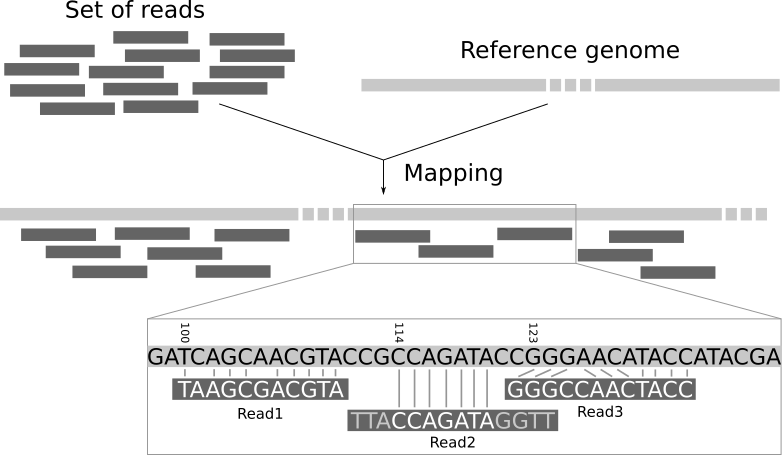
Figure Legend: Illustration of the mapping process. The input consists of a set of reads and a reference genome. In the middle, it gives the results of mapping: the locations of the reads on the reference genome. The first read is aligned at position 100 and the alignment has two mismatches. The second read is aligned at position 114. It is a local alignment with clippings on the left and right. The third read is aligned at position 123. It consists of a 2-base insertion and a 1-base deletion.

Tutorial Outline:

Read mapping has a few distinctive steps:

1. Trimming and filtering the input reads
2. Finding the appropriate reference genome
3. Actually mapping the reads
4. Calculating key statistics and summarizing the results

Removing adapters and low-quality reads with fastp

Because making sure our reads are high-quality is important but not the focus of this analysis, we are going to be using a program called Fastp that does the quality report generation as well as the trimming+filtering steps. More information can be found on the Fastp website: https://github.com/OpenGene/fastp. From the steps below, you can see that Fastp does pretty much the same operations as CutAdapt did last week!

Fastp does the following to our data :

• Filter out bad reads (too low quality, too short, etc.). The default sequence quality filter for Fastp is a Phred score of 15. Check back in your slides to see what base-calling accuracy this corresponds to!
• Cut low quality bases for per read from their 5’ and 3’ ends
• Cut adapters. Adapter sequences can be automatically detected, which means you don’t have to input the adapter sequences to trim them.
• Correct mismatched base pairs in overlapped regions of paired end reads, if one base is with high quality while the other is with ultra-low quality
• Several other filtering steps specific to different types of sequencing data.

Hands-On: Running fastp

1. Find the fastp - fast all-in-one preprocessing for FASTQ files tool.
2. Set single or paired reads to Paired Collection.
3. Make sure that you have selected the output of Faster Download and Extract Reads in FASTQ as the input.
4. Press Execute.
5. To view the resultant HTML report, you may need to download the file onto your computer (see below).

Examining the fastp results

Warning: Stop here and download the results!

Due to differences in the way that different browsers render HTML files, you may not be able to view the HTML file produced by fastp - fast all-in-one preprocessing for FASTQ files directly from the Galaxy interface itself. To get around this, you may need to download the HTML formatted report to your local computer first, and then click to open in your browser.

The HTML reports from filtering these data sets are FULL of information about the quality of these sequencing data sets.

For example, what percentage of the reads from SRR11954102 passed all of the filters of the fastp - fast all-in-one preprocessing for FASTQ files tool and remain in our data set? What about SRR12733957?

Solution

About 90% and 67%, respectively. To figure this out, first click on fastp on collection: HTML Report. Then, look into each of the data sets , and find the Filtering Result result section. For the SRR12733957 data set, this should roughly look like:

Filtering result
reads passed filters:	592.644000 K (67.755212%)
reads with low quality:	279.816000 K (31.990525%)
reads with too many N:	132 (0.015091%)
reads too short:	2.092000 K (0.239172%)

For the SRR11955102 data set, this should roughly look like:

reads passed filters:	2.650592 M (90.679913%)
reads with low quality:	270.274000 K (9.246396%)
reads with too many N:	2.154000 K (0.073691%)
reads too short:	0 (0.000000%)

Of the 10% of reads that were filtered from the data set SRR11955102, why were most of them filtered?

Solution

It looks like most of the reads that ended up getting removed from either data set were removed were removed because they were too low quality. We can tell this by looking again at the Filtering Result section, and seeing that about 9.2% out of the roughly 10% of the reads removed were removed as Reads with low quality.

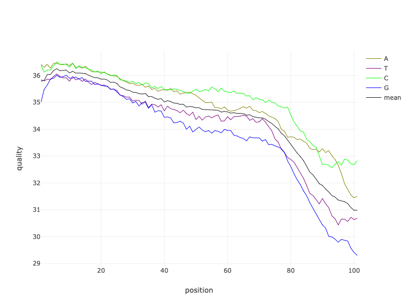
What are some of the main things we can learn from this plot of the quality of the Forward reads of the SRR11954102 BEFORE they were filtered?

Solution

A few of the things that I noticed are as follows.

• The reads are about 100bp long (see Position x-axis).
• The quality of the reads declines along their lengths, similar to the patterns described in the “Read Quality” lecture.
• Some bases towards the end of the read are lower than the cutoff quality score, especially for the any bases called as a G.
• What else do you notice?

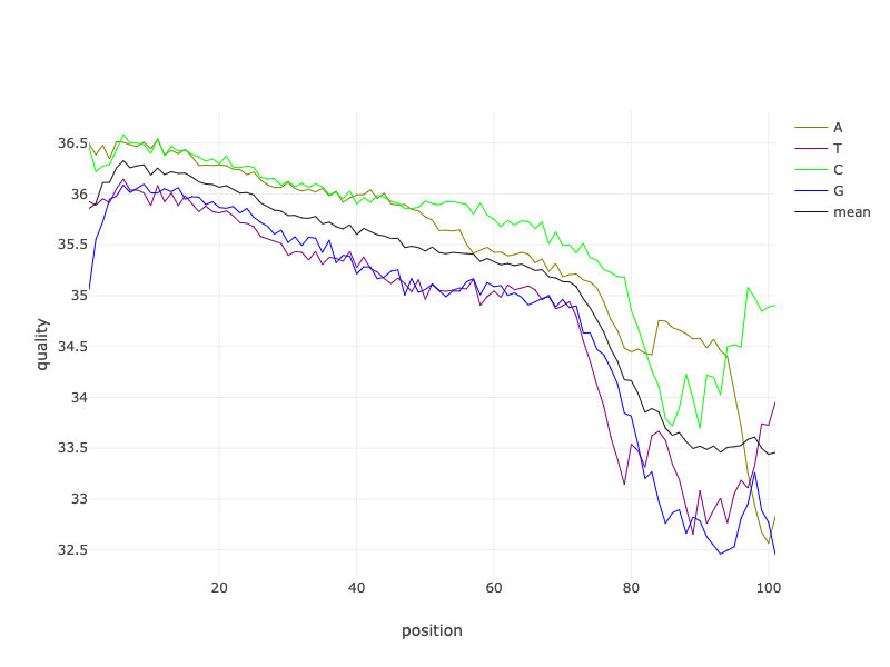
What are some of the main things we can learn from this plot of the quality of the Forward reads of the SRR11954102 AFTER they were filtered?

Solution

A few of the things that I noticed are:

• The reads are still about 100bp long (see Position x-axis).
• The quality of the reads still declines along their lengths.
• However, there is much less variation in quality along the read length.
• What else do you notice?

Getting the SARS-CoV-2 Reference Genome

In order to see what mutations the Boston strains of SARS-CoV-2 have accumulated relative to the original strain isolated from patients from Wuhan, China, we are going to map our filtered sequencing data to the full assembled genome of one of the original SARS-CoV-2 isolates, Wuhan-Hu-1. It has an accession ID of NC_045512.2, which you can search for on NCBI much like we did for the Boston samples to get more information. The Wuhan-Hu-1 reference genome is stored as a compressed FASTA file, rather than a FASTQ file.

Hands-On: Importing the reference genome from NCBI

1. Click the Upload Data button in the toolbar.
2. In the menu that pops up, click on Paste/Fetch Data
3. Copy and paste this address in the box: https://ftp.ncbi.nlm.nih.gov/genomes/all/GCF/009/858/895/GCF_009858895.2_ASM985889v3/GCF_009858895.2_ASM985889v3_genomic.fna.gz 4.Press Start. You can close the window now.

Mapping short-reads to the reference genome with BWA-MEM

Mapping against a pre-computed genome index:

Mappers usually compare reads against a reference sequence that has been transformed into a highly accessible data structure called genome index. Such indexes should be generated before mapping begins. Galaxy instances typically store indexes for a number of publicly available genome builds:

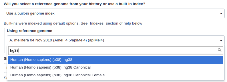
For example, the image above shows indexes for hg38 version of the human genome. You can see that there are actually three choices: (1) hg38, (2) hg38 canonical and (3) hg38 canonical female. The hg38 contains all chromosomes as well as all unplaced contigs. The hg38 canonical does not contain unplaced sequences and only consists of chromosomes 1 through 22, X, Y, and mitochondria. The hg38 canonical female contains everything from the canonical set with the exception of chromosome Y.

What if the pre-computed index does not exist?

If Galaxy does not have a genome you need to map against, you can upload your genome sequence as a FASTA file and use it in the mapper directly as shown below (Load reference genome is set to History). This is what we will need to do to use the Wuhan-Hu-1reference genome we just downloaded.

Hands-On: Map sequencing reads to reference genome

BWA-MEM is a widely used sequence aligner for short-read sequencing datasets such as those we are analysing in this tutorial.

1. Find the Map with BWA-MEM tool in the Tools panel.
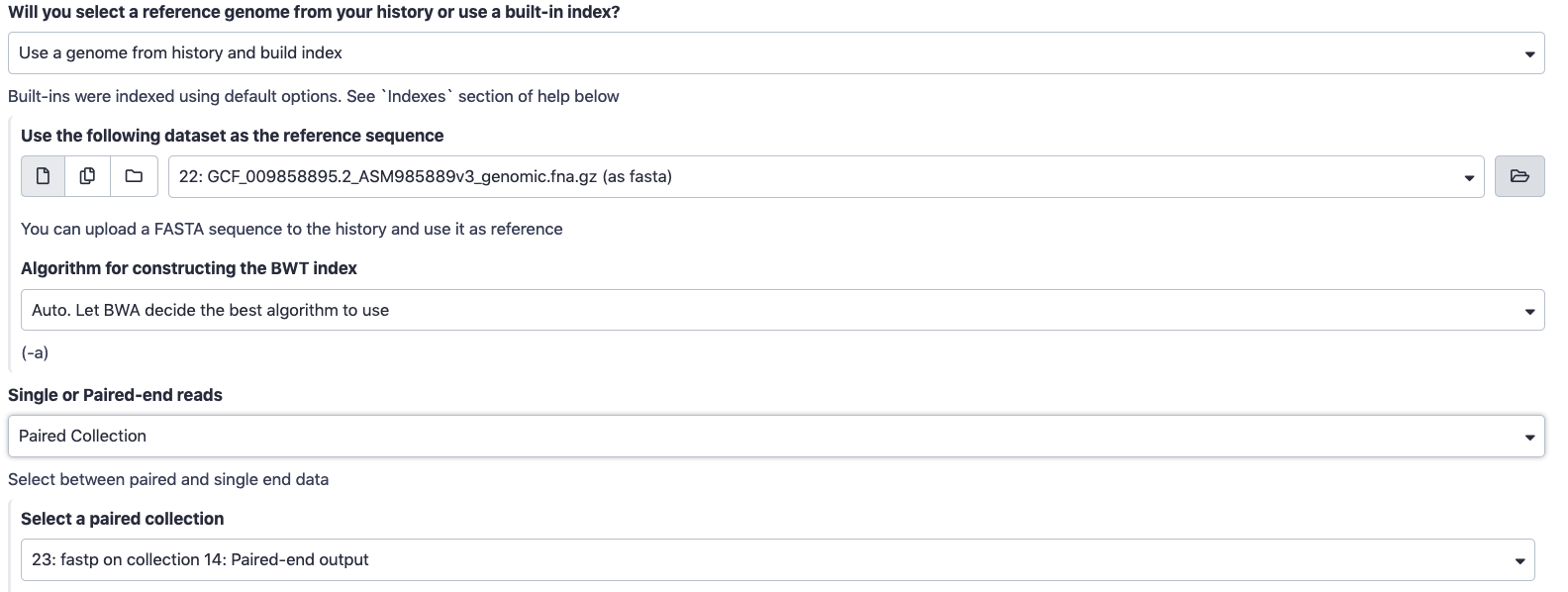
2. For the Will you select a reference genome from your history or use a built-in index? parameter, choose Use a genome from history and build index.
3. For the Use the following dataset as the reference sequence select the output from importing the reference genome in the last hands-on step.
4. For Single or Paired-End Reads select Paired Collection, and for Select a paired collection choose the output of fastp - fast all-in-one preprocessing for FASTQ files . Your window should now look something like this:
5. Set read groups information?: Do not set
6. Select analysis mode : 1. Simple Illumina Mode.
7. Click Execute! This may take a few minutes to run. .

Calculating Mapping Statistics

We often want to see how well our sequencing data mapped to the reference genome, which is useful for doing further troubleshooting and quality-control of our data. For example, if a very low proportion of sequencing reads map to your reference genome, one explanation could be that the sequencing data is not from the organism you thought it was! BWA-MEM technically outputs a Collection of BAM files, one for each sample. As we saw in the lecture on the SAM/BAM format, these are pretty big, complicated files. Luckily, there are utilities that can summrize the results!

What SAM alignment field would be used to help count up properly mapped reads?

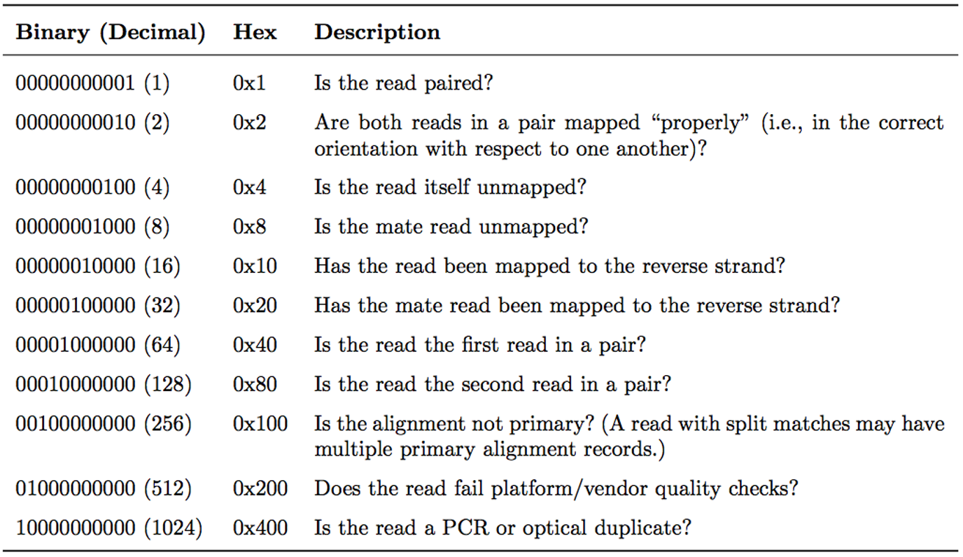
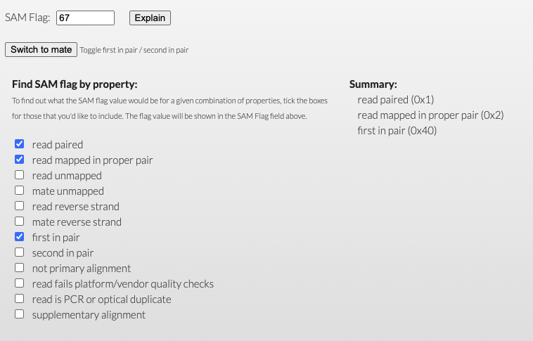
Looking back on our notes about the SAM/BAM format, we see that the **FLAG** alignment field contains information about the read’s mapping properties stored as bitwise flags.

For a program to count all of the reads that were Paired, mapped in a proper pair, and the R1 (first) read in the pair, the program would count up all instances of SAM Flag 67, or the the total decimal value of those conditions (1 + 2 + 64).

Several utilities exist online to help calculate and interpret these flags, such as: http://broadinstitute.github.io/picard/explain-flags.html.

You can also use read-mapping to troubleshoot this issue, by mapping your genome sequencing to the genome of potential contaminant organisms and removing the reads that map confidently to those genomes, OR keeping only those reads that confidently map to your genome of interest. For our actual input data set, we are just going to be calculating a few simple statistics about how many reads mapped to the genome.

Hands-On: Calculating mapping statistics

1. Find the BAM/SAM Mapping Stats tool in the Tools panel.
2. For Input .bam file select the folder icon and choose the output collection from Map with BWA-MEM .
3. Change Minimum mapping quality to 20, as this is the relevant mapping quality cutoff we will be using for our actual variant-calling step.
4. Press Execute!

Once the tool is done running, you can examine the results. The results from calculating mapping statistics for sample SRR11954102 look like this:

Total records:                          2659376

QC failed:                              0
Optical/PCR duplicate:                  0
Non primary hits                        0
Unmapped reads:                         2524130
mapq < mapq_cut (non-unique):           142
mapq >= mapq_cut (unique):              135104
Read-1:                                 67210
Read-2:                                 67894
Reads map to '+':                       59385
Reads map to '-':                       75719
Non-splice reads:                       135104
Splice reads:                           0
Reads mapped in proper pairs:           133752
Proper-paired reads map to different chrom:0

More Output Info:

• Total Reads (Total records) = Multiple mapped reads + Uniquely mapped
• Uniquely mapped Reads = read-1 + read-2 (if paired end)
• Uniquely mapped Reads = Reads map to ‘+’ + Reads map to ‘-‘
• Uniquely mapped Reads = Splice reads + Non-splice reads

Although this report gives us a lot of information, for the moment, we are very interested in the number of Unmapped Reads.

What percentage of this data set actually mapped to the SARS-CoV-2 reference genome?

Given all of this information in the report, we can do a pretty easy calculation to figure this out. We simply take 1 - Unmapped Reads/Total records. For this sample, we calculate 1 - (2524130/2659376) which ends up being approximately .051 or 5.1% of this data set. You would also get the same result by dividing the number of unique mapped reads (135104) by the Total records.

Perhaps surprisingly, only a few percent of our input data set mapped to the SARS-CoV-2 reference genome. However we are not too worried, given the process to used to collet this sample (nasal swab), and that this still leaves us with over 130k reads to map to the small Sars-Cov-2 genome

Calculating Genome Coverage Using the Mapping Results: Do we have enough mapped data?

We can in fact calculate a quick approximation of the *coverage for the mapped portion SRR11954102 data set, that is, how many times over does this data cover the Wuhan-Hu-1 reference genome?

We know that there are 135104 uniquely mapped, useable reads, and that after filtering, the mean length of the reads was 86 bp (see fastp report). We multiply these together to get the approximate total number of bases in our data set: 11,618,944 bp. Then, we divide this by the SARS-Cov-2 genome size, 29,903 bp.

This gives us a coverage of approximately 388x, which in words means that our remaining mapped data should cover the reference genome 388 times, which is more than enough to carry out the rest of the variant calling analysis!

Key Points

• Read mapping is the process of placing reads on the reference genome

• You can calculate important statistics and diagnose issues using results from read mapping