Hands On: Variant Calling in Galaxy
Overview
Teaching: min
Exercises: 30 minQuestions
Objectives
Identify major steps in a variant-calling workflow and their associated file types
Operate on a collection of data from two samples to perform a variant-calling workflow
Add functional information to called variants
Manipulate the output from a variant-calling workflow to answer biologically relevant questions
Warning: Results may vary!
Your results may be slightly different from the ones presented in this tutorial due to differing versions of tools, reference data, external databases, or because of stochastic processes in the algorithms.
Tutorial Preview: Steps in Variant Calling
As you learned from this week’s lectures, variant-calling is the process of identifying small variations in the sequence data of an individual sample, generally in comparison to a standard reference that we can compare to multiple samples.
So far, you have done the following:
- Obtaining sequence data.
- Identifying samples of interest from their metadata
- Using the Galaxy interface to load the sequence data from these samples into your workspace.
- Pre-processing the data.
- Generating and examining sequence-quality reports
- Filtering and trimming your reads
- Mapping the data to a reference genome
In this tutorial, you will learn how to do the following:
- Quality control of the mapped reads to prepare for calling variants
- Removing duplicates
- Re-aligning reads and adding indel qualities
- Calling variants
- Annotating variants with functional information
- Post-processing data
- Collapsing multiple data sets
- Manipulating text files to answer questions
Preparing the results of read-mapping for variant-calling
In the next few steps, we will be processing the output from in order to make the variant calling step go as smoothly as possible:
- Removing duplicates
- Re-aligning reads
- Adding indel qualities.
We will be feeding the output of one step right into the next one as input, which is very common for multi-step bioinformatics analyses.
Process Mapping Results Step 1: Removing duplicates
As you can probably guess from the name of this step, this removes duplicate sequences originating from library preparation artifacts and sequencing artifacts. It is important to remove this artifactual sequences to avoid artificial sequences to avoid artificial overrepresentation of particular single molecules.
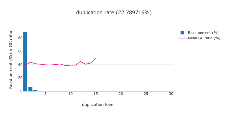
What percentage of reads were duplicated in the raw SRR11954102? What about in the original SRR12733957 data set? Hint: This information can be found in output that we already have in our history.
Solution
Take a look back at the HTML report generated by the tool. There is a
Duplicationsection available that looks like the following forSRR11954102:We can see form this graph that most sequences are present in only one copy (duplication level of 1), meaning this sample has a low overall duplication level (2.3%) - only 2.3% of sequences are duplicates of each other.
If we look at
SRR12733957, we see that this level is much greater (~ 22.8%).
Measuring duplication levels
Note that the levels of duplication are inferred based on read sequence similarity alone because the short-read data had not been mapped to a reference genome yet. The following MarkDuplicates step will remove duplicate copies of reads while incorporating information about their mapped position on the reference genome.
Hands-On: Removing Duplicates
Find the tool. The full title should be something like
Mark Duplicates examine aligned records in BAM datasets to locate duplicate molecules.Run this tool with the following modified parameters:
- Select SAM/BAM dataset or dataset collection: Click the folder icon and choose output of .
- If true do not write duplicates to the output file instead of writing them with appropriate flags set set to
Yes. This switch tells MarkDuplicates to not only mark which short reads are duplicates of one another, but to also remove them from the output file.
Process Mapping Results Step 2: Re-aligning Reads
Next, we will run tool that re-aligns read to the reference genome, while correcting for misalignments around insertions and deletions. This is required in order to accurately detect variants.
Hands-On: Re-aligning Reads
Find the tool. Run with the following parameters:
- Reads to re-align should be set to the output of .
- Choose the source for the reference genome:
History, and the Reference should be the same input reference genome as for the step.- Check that Advanced Options: “How to handle base qualities of 2?” is set to
Keep Unchanged.
Process Mapping Results Step 3: Adding Indel Qualities
This step adds indel qualities into our alignment file. These are a measurement of how certain lofreq is that an insertion or deletion is “real”, and not just an artifact of sequencing or mapping. This is necessary in order to call variants.
Hands-On: Add indel qualities with lofreq
Find the tool. Run with the following parameters:
- Reads:
realigned, and select output of .- Indel calculation approach:
Dindel.- Choose the source for the reference genome:
History, and the Reference should be the same input reference genome as for the step.
Now we are ready to actually call our variants!
The Actual Variant-Calling
Hands On: Call variants using lofreq
Find and run with the following parameters:
- Input reads in BAM format: select output of .
- Choose the source for the reference genome:
History, and the Reference should be the same input reference genome as for the step.- Call variants across:
Whole reference- Types of variants to call:
SNVs and indels- Go into Variant calling parameters: Configure settings
- In Coverage:
- Minimal coverage:
50- In Base-calling quality:
- Minimum baseQ:
30- Minimum baseQ for alternate bases:
30- In Mapping quality:
- Minimum mapping quality:
20- Variant filter parameters: Preset filtering on QUAL score + coverage + strand bias (lofreq call default)
Once those are all set, click
Execute!
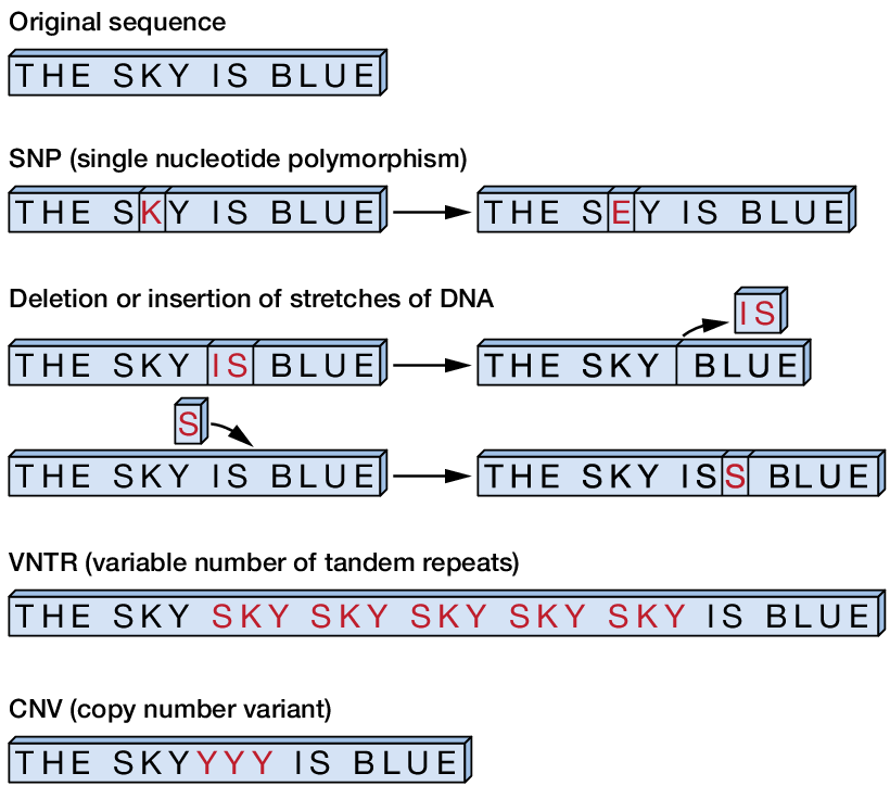
Once this has run, we have now found many places in the genome where your sample differs from the reference genome - this is where we are right now after calling variants. Variants can be categorized as follows:
- SNP (Single-Nucleotide Polymorphism) Reference = ‘A’, Sample = ‘C’
- Ins (Insertion) Reference = ‘A’, Sample = ‘AGT’
- Del (Deletion) Reference = ‘AC’, Sample = ‘C’
- MNP (Multiple-nucleotide polymorphism) Reference = ‘ATA’, Sample = ‘GTC’
- MIXED (Multiple-nucleotide and an InDel) Reference = ‘ATA’, Sample = ‘GTCAGT’

Figure Caption: Examples of types of sequence variants. For now, we are not looking specifically for tandem repeats and copy number variants. From Philibert et al. 2014.
Getting ready to interpret our variant-calling results
So, we have variant-calling results, but they are not particular useful, for us as humans, to look at yet. So, we are going to add information about the biological relevance of variants by annotating variant effects, and then creating an organized table of variants by extracting fields from the table of annotation information. Finally, we will collapse the collection of final, annotated results for the two datasets we originally downloaded from NCBI SRA to make them even easier for us to use.
To annotate variant effects, we are using software called SnpEff (i.e. “SNP effects”), which annotates and predicts the effects of genetic variants (such as amino acid changes). Using our variant-calling, we now have a list of genetic variants in our Boston SARS-CoV-2 samples as compared with the Wuhan-Hu-1 reference genome. But say want to know more about these variants than just their genetic coordinates. E.g.: Are they in a gene? In an exon? Do they change protein coding? Do they cause premature stop codons? SnpEff can help you answer all these questions. The process of adding this information about the variants is called “Annotation”.
SnpEff provides several degrees of annotations, from simple (e.g. which gene is each variant affecting) to extremely complex annotations (e.g. will this non-coding variant affect the expression of a gene?).
Conveniently, there is a special version of SnpEff that is specifically calibrated for and connected to a database of known variant effects in SARS-CoV-2 genomes, which we will be using below.
Hands-On: Annotate variant effects with SnpEff
Find and run and modify the following parameters:
- Input reads in VCF format: select output of .
- Select annotated Coronavirus Genome is
NC045512.2, which is the annotated version of the reference genome we have been using throughout.- Output format:
VCF (only if input is VCF).- Create CSV report Useful for downstream analysis (-csvStats):
Yes- “Filter out specific Effects”:
No.
Hands-On: Create human-readable table of variants with SnpSift
Find and run and modify following the parameters:
- Variant input file in VCF Format: select output of .
- Make sure Fields to Extract is as follows:
CHROM POS REF ALT QUAL DP AF SB DP4 EFF[*].IMPACT EFF[*].FUNCLASS EFF[*].EFFECT EFF[*].GENE EFF[*].CODONFeel free to copy and paste!- One effect per line:
Yes.- empty text field:
.(just a period).
Hands-On: Collapse data into a single dataset
Find and run and modify following the parameters:
- Collection of files to collapse: select output of .
- Keep one header line:
Yes- Prepend File name:
Yes- Where to add dataset name:
Same line and each line in dataset.
You can see that this tool takes lines from all collection elements (in our case we have two), add element name as the first column, and pastes everything together. So if we have a collection as an input:
Example of Collapse:
Let’s say our collection element for
SRR11954102is the following:NC_045512.2 84 PASS C T 960.0 28 1.0 0 0,0,15,13 MODIFIER NONE INTERGENIC NC_045512.2 241 PASS C T 2394.0 69 0.971014 0 0,0,39,29 MODIFIER NONE INTERGENICAnd that our item for
SRR12733957, we had:NC_045512.2 241 PASS C T 1954.0 63 0.888889 0 0,0,42,21 MODIFIER NONE INTERGENIC NC_045512.2 823 PASS C T 1199.0 50 0.76 3 5,6,13,26 LOW LOW LOWWe will have a single dataset as the output, with an added column containing the dataset ID taken from the collection element names.
SRR11954102 NC_045512.2  84 PASS  C T  960.0  28  1.0       0 0,0,15,13 MODIFIER  NONE  INTERGENIC
SRR11954102 NC_045512.2 241 PASS  C T 2394.0  69  0.971014  0 0,0,39,29 MODIFIER  NONE  INTERGENIC
SRR12733957 NC_045512.2 241 PASS  C T 1954.0  63  0.888889  0 0,0,42,21 MODIFIER  NONE  INTERGENIC
SRR12733957 NC_045512.2 823 PASS  C T 1199.0  50  0.76      3 5,6,13,26 LOW       LOW   LOW
What is in our final, collapsed result file?
So, now we have a file containing our called variants, and their potential biological significance, for both of our input data sets, SRR12733957 a sequencing run from a sample collected from Boston in April 2020, and SRR11954102, collected from Boston in May 2020. This is a file that you could manipulate in Excel or R if you already use one of those programs for statistics, but for this exercise, we are going to continue to work in Galaxy for the sake of consistency.
Here are the columns of information that are present in our final output from .
This is what the first two lines of our actual output datat set looks like:
Sample	CHROM	POS	REF	ALT	QUAL	DP	AF	SB	DP4	EFF[*].IMPACT	EFF[*].FUNCLASS	EFF[*].EFFECT	EFF[*].GENE	EFF[*].CODON
SRR11954102	NC_045512.2	84	C	T	7114.0	208	0.975962	0	0,1,102,105	MODIFIER	NONE	intergenic_region	CHR_START-ORF1ab	n.84C>T
SRR11954102	NC_045512.2	160	G	T	144.0	254	0.031496	14	166,77,10,0	MODIFIER	NONE	intergenic_region	CHR_START-ORF1ab	n.160G>T
The first column, Sample, has been added by SnpSift. The rest of these first few columns, CHROM - QUAL, are standard for variant-call-format files (VCFs). DP - DP4 which provide more information about the read information that supports the called variant, are also commonly found in the output of variant-calling software:
| Column | Description |
|---|---|
| Sample | Sample Name (added by SnpSift) |
| CHROM | Chromosome of reference, not really applicable for viral genomes |
| POS | Base pair position in reference genome |
| REF | The reference allele (what the reference genome has at this position) |
| ALT | The alternate allele (what this sample has at this position) |
| QUAL | Phred quality score for confidence in the variant call |
| DP | Combined depth across samples |
| AF | Allele frequency for each ALT allele |
| SB | Strand bias at position |
| DP4 | Depth of the reference forward, reference reverse, alternate forward, alternate reverse bases |
The rest of the columns contain information given to us by the SnpEff annotation process:
| Column | Description |
|---|---|
| EFF[*].IMPACT | Estimate of how strong of an impact this variant is predicted to have on on protein function. |
| EFF[*].FUNCLASS | Type of mutation: NONE, SILENT, MISSENSE, NONSENSE |
| EFF[*].EFFECT | Actual effect of this variant on protein coding (i.e. frameshift or misssense) |
| EFF[*].GENE | Gene name if in coding region. |
| EFF[*].CODON | Codon change: old_codon > new_codon |
Notes about some categories
EFF.IMPACT
MODIFIERalleles: Usually non-coding variants or variants affecting non-coding genes, where predictions are difficult or there is no evidence of impact.EFF.GENE names: Most genes in this SARS-CoV-2 reference genome are named simply as open reading frames (ORFs).
Let’s answer some questions about our data using Galaxy!
We are going to be using Galaxy utilities to do some tabulating and counting. Note that in this collapsed output, each line represents a variant site and a predicted effect. Some variants will have multiple effects. We are more interested in quantifying these different effects, so we will be using various tools to count the number of rows that pertain to different conditions.
Hands-On: Using the Count tool
Suppose we want to know: How many effects caused by variants were found in each sample?
We could look back at the uncollapsed files of each sample and see how many line they have, but we can also perform a single operation on the final file to get the results. Find and run and modify following the parameters:
- From Dataset: Our output from .
- Count occurrences of values in column(s):
Column 1.- Leave Delimited By and How should the results be sorted as is right now.
Viewing the small output file, you should see that there are two lines, which represent the number of times either of the SRA IDs appear in the first column.
From this output, we can see that there are 759 variant effects found in
SRR11954102and 427 inSRR12733957.How many effects in each data set are predicted to have a HIGH impact?
Run the again on the same input file as above, but this time, add the column containing the
EFF[*].IMPACTinformation (should becolumn 11) as a column for counting occurrences.Look at the output file. This time it has counted occurrences of each unique pairing of a Sample ID and a
EFF[*].IMPACTlevel:If we look just at the rows where
EFF[*].IMPACT = HIGH, we can see thatSRR11954102has 97 of these effects, andSRR12733957has 49.
Hands-on: Using the Filter tool
Suppose we want to know: What variant-associated effects are associated with the Spike Protein (S-protein), and perform operations just on those rows?
- Find the tool.
- Set the Filter input: Our output from .
- Set With following condition :
c14=='S'.
- This is telling the tool to only return rows where the 14th column of our collapsed data set,
EFF[*].GENEequals"S", the shorthand name for the Spike protein.- The double equal sign
==is necessary to specify that we want this code to test whether two values are equal. You will learn more aboutlogical operatorswhen we look at data in RStudio in a future lesson.- Set Number of Header Lines to Skip to
1, since our data set has one line of column names.- Take a look at the output file . It should have the same columns as the input, but limited to rows where the value of
EFF[*].GENEisS.- The helpful summary of the output file tells us the following:
Filtering with c14=='S', kept 4.04% of 1187 valid lines (1187 total lines), and that the file is 48 lines long. Because this 48 includes the header, we know that there are 47 Spike protein mutations in our data set!How many of these Spike protein effects can be found in each sample?
There are several ways to do this, but one way uses the same tool as above.
This time, make sure that the From Dataset variable is set to the output of Filter that we just generated.
As before, we will count occurrences in
Column 1.The output should have just two lines with the number Spike protein mutations in each of the two input sequencing data sets:
29	SRR11954102
18	SRR12733957
Hands-On: Finding one particular mutation using the
Select linestoolSuppose we want to know: Do either of our samples have one of the diagnostic sequence changes associated with the more transmissible B.1.1.7 SARS-CoV-2 strain? We know the B.1.1.7 lineage contains a nonsense mutation (changing a legitimate codon specifying an amino acid to a stop codon) in ORF8a, at nucleotide
27972.Do we have any variants called at position
27972in our data set?One solution is to use the tool with the following parameters:
- Make sure our final, collapsed is listed in the Select lines from field of the tool form.
- The expression we are looking for is the nucleotide number, simply
27972. Our output will look like the following:SRR11954102 NC_045512.2 27972 C T 226.0 368 0.032609 0 103,252,4,9 HIGH NONE stop_gained ORF8 c.79C>T SRR12733957 NC_045512.2 27972 C T 1067.0 253 0.162055 0 37,169,7,40 HIGH NONE stop_gained ORF8 c.79C>TYou can see that both of our data sets have a variant at position
27972, and that both result in astop_gainedmutation inORF8, just as in the B.1.1.7 lineage. This is interesting because these datasets were collected well before B.1.1.7 became widely spread, particularly in the United States!
Exporting our final data set
One way that we can make this data set even more useful is to export the final collapsed tabular dataset into a CSV file so that ourselves and other researchers can import it into something like Excel or Rstudio, allowing us to conducted even more complex analyses and visualizations. So, as the final step in this pipeline, we are going to do just that!
Hands-On: Converting the collapsed data set to CSV for export
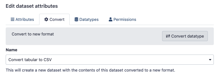
Click on the pencil icon for the Collapse Collection data item in your History.
This should open a
Edit Dataset Attributesmenu.Click on the
Converttab, and clickConvert datatype.This menu is context-sensitive, so because we are working with a
Tabulardataset, the only conversion option should beConvert tabular to CSV.
Click
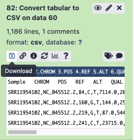
Convert Datatype. This will create a new dataset with the contents of this dataset, just converted into a CSV.Find the disk image icon option for this new item, and click it to download - make sure to change the default filename from Galaxy to something clearer!
- Try opening the file in Excel or your spreadsheet tool of choice!
Key Points
Variant-calling is the process of identifying small variations in the sequence data
Variant-calling is a multistep pipeline that builds upon steps you have already encountered: Quality control and Mapping.


