Hands On: Creating Counts from Mapped Reads

Overview

Teaching: min
Exercises: 30 min

Questions

Objectives

• Learn how RNA-seq reads are converted into counts

• Learn different metrics for troubleshooting RNAseq expression data

• Utilize an imported Galaxy Workflow that performs QC on the mapped read data and counts

Heads up: Results may vary!

It is possible that your results may be slightly different from the ones presented in this tutorial due to differing versions of tools, reference data, external databases, or because of stochastic processes in the algorithms.

What is counting?

The alignment produced a set of BAM files, where each file contains the read alignments for each sample. In the BAM file, there is a chromosomal location for every read that mapped. Now that we have figured out where each read comes from in the genome, we need to summarise the information across genes or exons. The mapped reads can be counted across mouse genes by using a tool called featureCounts. featureCounts requires gene annotation specifying the genomic start and end position of each exon of each gene. For convenience, featureCounts contains built-in annotation for mouse (mm10, mm9) and human (hg38, hg19) genome assemblies, where exon intervals are defined from the NCBI RefSeq annotation of the reference genome.

Reads that map to exons of genes are added together to obtain the count for each gene, with some care taken with reads that span exon-exon boundaries. The output is a count for each Entrez Gene ID, which are numbers such as 100008567. For other species, users will need to read in a data frame in GTF format to define the genes and exons. Users can also specify a custom annotation file in SAF format. Doing so is a bit outside the scope of this course!

Hands-on: Count reads mapped to genes with featureCounts

1. Run featureCounts Make sure that you have chosen the exact right version of this tool 2.0.1+galaxy1 using the version menu at the top of page. .
2. Modify the following parameters to the following, IN THIS ORDER:
   • Select "featureCounts built-in" for the “Gene annotation file”. This will appear to not do anything.
   • “Alignment file”: Choose the collection option, and it should by default choose the output of HISAT2. Select this output collection if it is not already selected.
3. At this point, under “Gene annotation file”: featureCounts built-in, “Select built-in genome” should be mm10. If not, mm10 should at least be available to select.
4. Applying the same logic as the last time we ran MultiQC, run MultiQC with the appropriate options for the output of featureCounts.
5. Add a tag #featurecounts to the Webpage output from MultiQC and inspect the webpage.

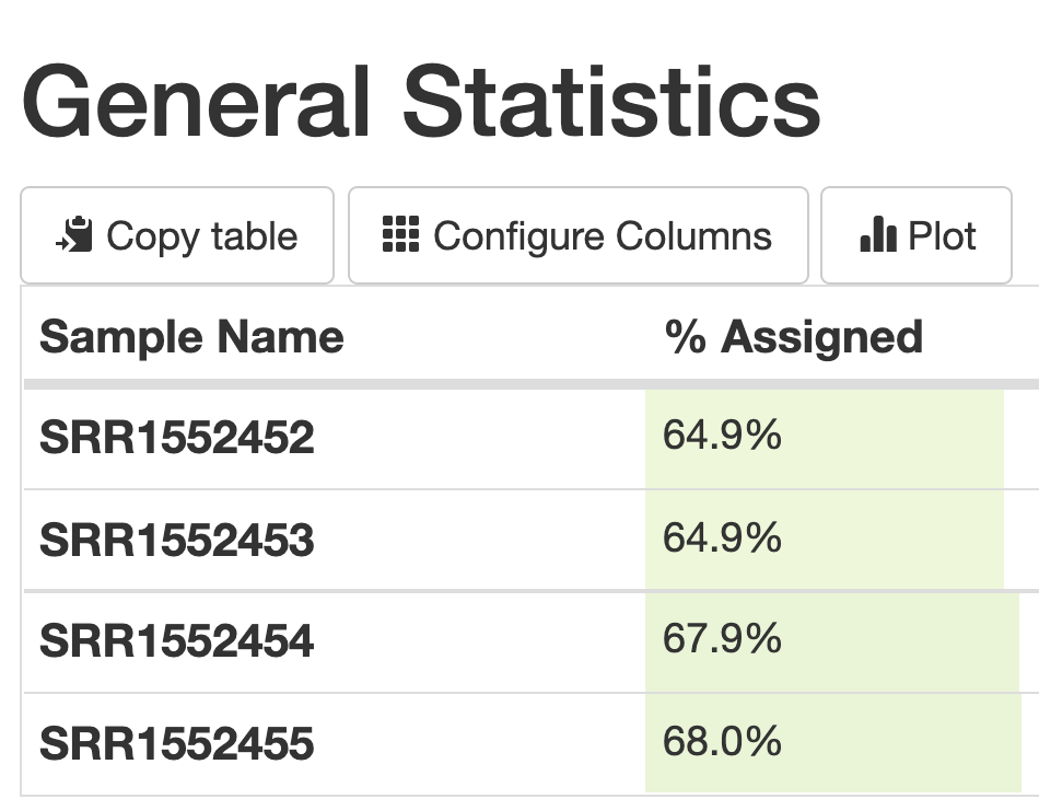
We can see from the summary that about 65% of each data set was able to be assigned uniquely to actual coding regions of the genome (exons).

Note: featureCounts parameters

In this example we have kept many of the default settings, which are typically optimised to work well under a variety of situations. For example, the default setting for featureCounts is that it only keeps reads that uniquely map to the reference genome. For testing differential expression of genes, this is preferred, as the reads are unambigously assigned to one place in the genome allowing for easier interpretation of the results. Understanding all the different parameters you can change involves doing a lot of reading about the tool that you are using, and can take a lot of time to understand! We won’t be going into the details of the parameters you can change here, but you can get more information from looking at the tool help.

Finding out more about a gene using the Entrez ID

The counts for the samples are output as a tabular file - take a look at one! The numbers in the first column of the counts file represent the Entrez gene identifiers for each gene, while the second column contains the counts for each gene for the sample. According to NCBI, Entrez gene IDs “provide unique integer identifiers for genes and other loci (such as officially named mapped markers) for a subset of model organisms.”

They are extremely useful for being sure that you are referring to the exact same gene in the exact same model organism as someone else is!

Hands-On: Finding out more about a gene

1. Let’s look at the first gene in the mapping output for SRR1552452. For me (it may vary), it is an ID number of 497097, and there are 65 reads which have mapped to it.
2. Go to https://www.ncbi.nlm.nih.gov/.
3. In the search bar, enter 497097 and choose Gene in the dropdown menu next to the search bar.
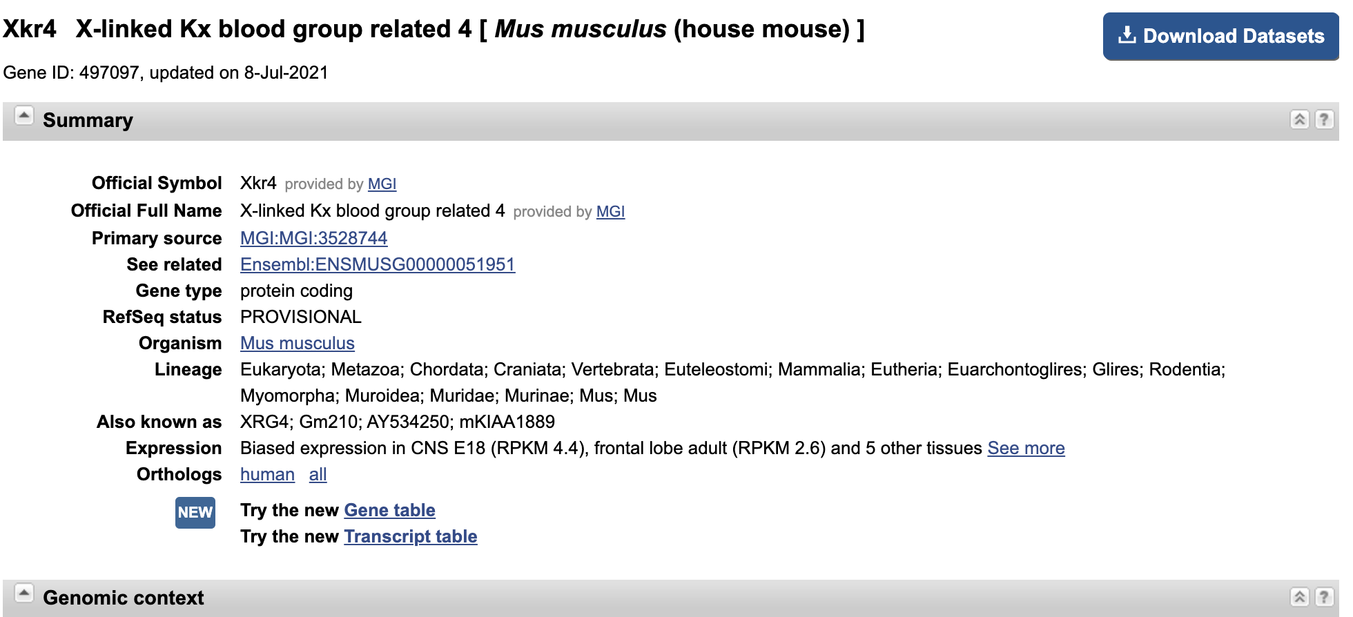
4. This number can be found in multiple databases, so click on the Gene results.
5. We can see that this gene is Xkr4, or X-linked Kx blood group related 4.
6. This page also serves as a portal for A LOT of other information about the gene, which may come in handy later:

Create Count Matrix

The counts files are currently in the format of one file per sample. However, it is often convenient to have a count matrix. A count matrix is a single table containing the counts for all samples, with the genes in rows and the samples in columns. The counts files are all within a collection so we can use the Galaxy Column Join on multiple datasets tool to easily create a count matrix from the single counts files.

Hands-on: Create count matrix with Column Join on multiple datasets

Column Join on Multiple Data Sets with the following parameters:

• “Tabular files”: Counts (output of featureCounts.
• “Identifier column”: 1.
• “Number of header lines in each input file”: 1.
• “Add column name to header”: No. The Count Matrix should look something like this, and have approximately 21,000 lines of data: . For the sake of downstream analyses, rename this output file countdata as a shorthand.

How do we interpret the counts for gene 100012?

As you can see from the screenshot above, the read counts for each sample for this gene are 0,0,0 and 0, respectively. This means that in our analysis, there are no reads associated with this particular gene in the mouse genome for any of our samples. This gene will essentially be out of consideration for downstream analyses because it has no expression level (0) for all of the samples.

Doing QC of the Read Counts Using an Imported Workflow

There are several additional QCs we can perform to better understand the data, to see if it’s good quality. These can also help determine if changes could be made in the lab to improve the quality of future datasets.

We’ll use a prepared workflow to run the first few of the QCs below. This will also demonstrate how you can make use of Galaxy workflows to easily run and reuse multiple analysis steps.

The imported workflow will do the following automatically:

• Run the Infer Experiment tool
• Run the MarkDuplicates tool (we used this tool during variant-calling).
• Run the IdxStats tool.
• Generate a MultiQC report

Galaxy Workflows can be imported to your history directy from a URL if you know the right URL. We are going to use this option right now. You can then edit the workflow if you’d like to add other steps.

This workflow will also involve uploading a BED file associated with the mm10 mouse genome that we have been using. We will not be using this format in other tutorials so we will not need to go into much depth about what they contain.

The BED format (Browser Extensible Data format) provides a flexible way to encode gene regions. Lines in a BED file have three required fields:

• chromosome ID
• start position (0-based)
• end position (end-exclusive)
• There can be up to and nine additional optional fields, but the number of fields per line must be consistent throughout any single set of data.

Hands-On: Importing the QC Workflow

1. Click on Workflow on the top menu bar of Galaxy. You will see a list of all your workflows.
2. Click on the Import icon at the top-right of the screen.
3. Copy and paste the following URL into the Archived Workflow URL box:

   https://training.galaxyproject.org/training-material/topics/transcriptomics/tutorials/rna-seq-reads-to-counts/workflows/qc_report.ga
   

1. Click the Import Workflow button.
2. You should now have a new workflow entitled QC Report (imported from uploaded file) in your list of workflows.

Hands-on: Running the QC Report workflow

1. Import this file as a BED file using the Upload Data tool.

   https://sourceforge.net/projects/rseqc/files/BED/Mouse_Mus_musculus/mm10_RefSeq.bed.gz/download
   

2. Go back to your Workflow page.
3. Click on the Run Workflow button next to the workflow you just imported.
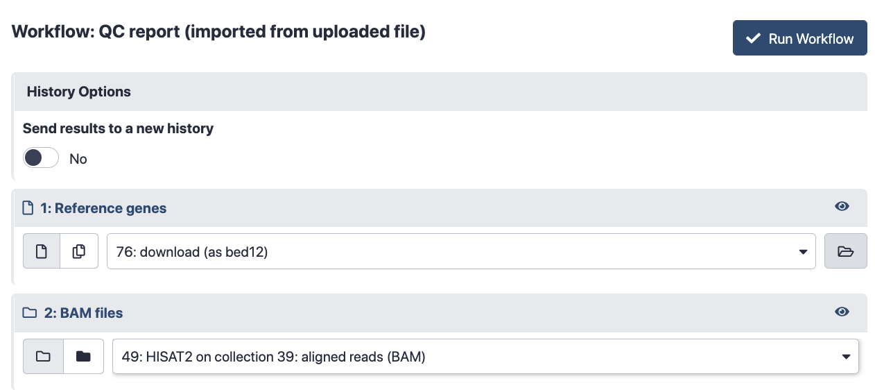
4. Run Workflow QC Report using the following parameters. You may need to click Expand to full workflow form to see these options:
   • “Send results to a new history”: No.
   • “1: Reference genes”: the imported RefSeq BED file.
   • “2: BAM files”: The aligned reads (BAM) created by HISAT2 . For reference, my workflow page looked like this when I was ready to run the workflow (Your History Item numbers will likely differ):

1. Click the Run Workflow button at the top-right of the screen. You may have to refresh your history to see the queued jobs.
2. Inspect the Webpage output from MultiQC once all of the jobs are done running.

Interpreting the QC Report output

Now what?

You do not need to run the hands-on steps below. They are just to show how you could run the tools individually and how we can use the output to learn more about our mapping and count results. If the imported workflow ran correctly, you should see all of the figures you discussed in the final output MultiQC report! Just one of the many reasons that using reproducible workflows in Galaxy is awesome.

Strandedness

RNAs that are typically targeted in RNA-Seq experiments are single stranded (e.g., mRNAs) and thus have polarity (5’ and 3’ ends that are functionally distinct). During a typical RNA-Seq experiment the information about strandness is lost after both strands of cDNA are synthesized, size selected, and converted into a sequencing library. However, this information can be quite useful for the read counting step, especially for reads located on the overlap of 2 genes that are on different strands. As far as we know this data is unstranded, but as a sanity check you can check the strandness. This information should be provided with your FASTQ files, ask your sequencing facility! If not, try to find it on the site where you downloaded the data or in the corresponding publication.

Figure: Read1 will be assigned to gene1 located on the forward strand but Read2 could be assigned to gene1 (forward strand) or gene2 (reverse strand) depending if the strandness information is conserved.

This workflow uses the RSeQC Infer Experiment tool to “guess” the strandness. This tool takes the BAM files from the mapping, selects a subsample of the reads and compares their genome coordinates and strands with those of the reference gene model (from an annotation file). Based on the strand of the genes, it can gauge whether sequencing is strand-specific, and if so, how reads are stranded (forward or reverse):

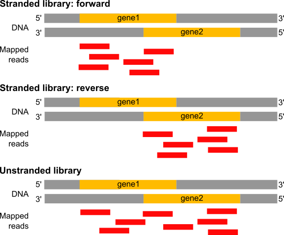Figure: In a stranded forward library, reads map mostly on the genes located on forward strand (here gene1). With stranded reverse library, reads map mostly on genes on the reverse strand (here gene2). With unstranded library, reads maps on genes on both strands.

RSeQC Infer Experiment tool generates a file with information on:

• Paired-end or single-end library.
• Fraction of reads failed to determine.
• 2 lines:
  • For single-end:
    • Fraction of reads explained by "++,--": the fraction of reads that assigned to forward strand.
    • Fraction of reads explained by "+-,-+": the fraction of reads that assigned to reverse strand.
  • For paired-end:
    • Fraction of reads explained by "1++,1--,2+-,2-+": the fraction of reads that assigned to forward strand.
    • Fraction of reads explained by "1+-,1-+,2++,2--": the fraction of reads that assigned to reverse strand.

If the two “Fraction of reads explained by” numbers are close to each other, we conclude that the library is not a strand-specific dataset (or unstranded).

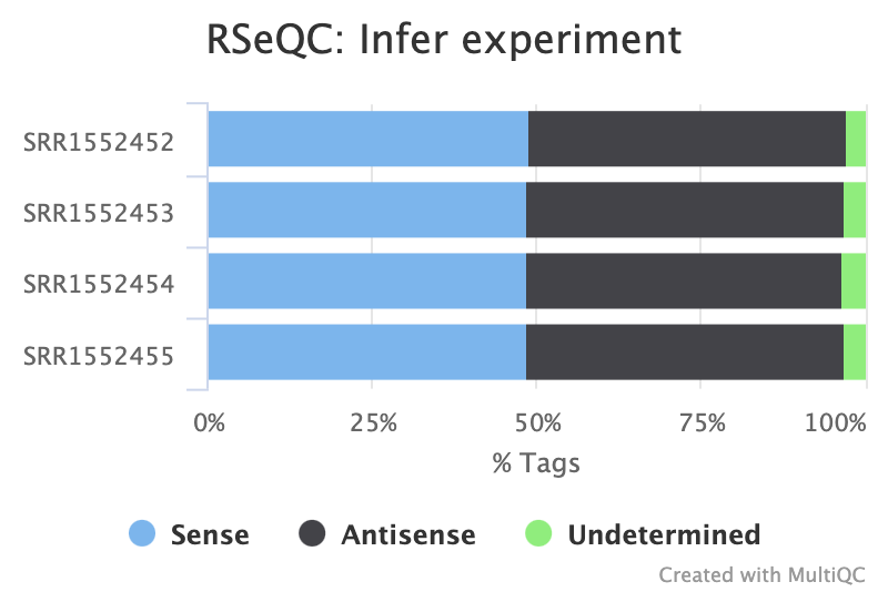Figure: Infer Experiment Summary Plot for our four samples.

Do you think the data is stranded or unstranded?

It is unstranded as approximately equal numbers of reads have aligned to the sense and antisense strands.

Read Duplication

Duplicate reads are usually kept in RNA-seq differential expression analysis as they can come from highly-expressed genes but it is still a good metric to check. A high percentage of duplicates can indicate a problem with the sample, for example, PCR amplification of a low complexity library (not many transcripts) due to not enough RNA used as input. FastQC gives us an idea of duplicates in the reads before mapping (note that it just takes a sample of the data). We can assess the numbers of duplicates in all mapped reads using the Picard MarkDuplicates tool. Picard considers duplicates to be reads that map to the same location, based on the start position of where the read maps. In general, we can consider it normal in an RNAseq library to obtain up to 50% of duplication.

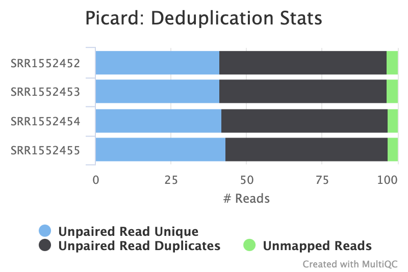
Which two samples have the most duplicates detected?

It is hard to tell looking at the summary figure alone. Looking at the raw MultiQC Stats output, samples SRR1552452 and SRR1552453(both from pregnant mice) have slightly higher level of duplication than the samples from lactating mice.

Reads Mapped Per Chromosome

You can check the numbers of reads mapped to each chromosome with the Samtools IdxStats tool. This can help assess the sample quality, for example, if there is an excess of mitochondrial contamination. It could also help to check the sex of the sample through the numbers of reads mapping to the X or Y or to see if any chromosomes have highly expressed genes.

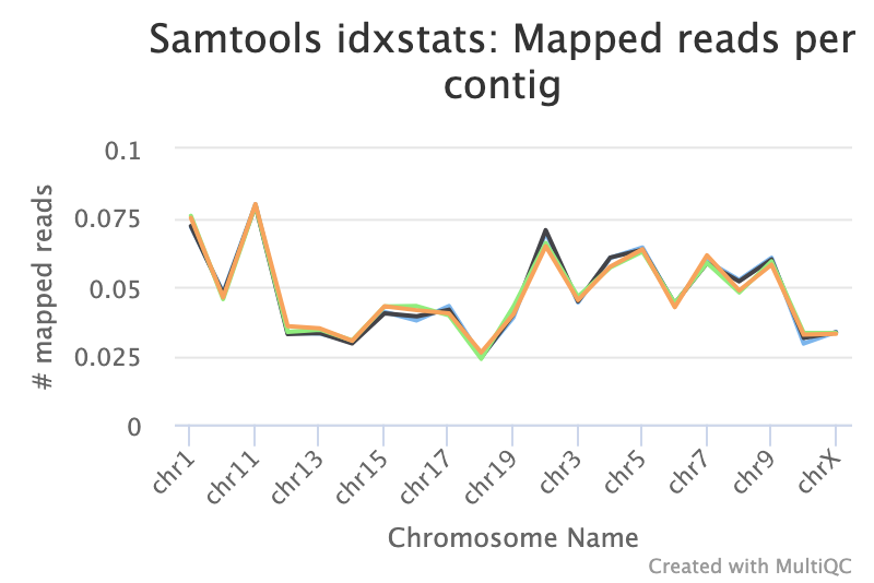Figure: IdxStats Chromosome Mappings, per chromosome for all chromosomes.

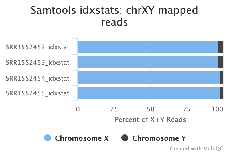Figure: IdxStats XY Mappings.

Interpreting Per-Chromosome Plots

1. What do you notice aboutg the overall distribution of reads mapped to each chromosome?
2. Are the samples male or female? (If a sample is not in the XY plot it means no reads mapped to Y).

Solution

1. Samples appear to have roughly the same pattern of distribution across the chromosomes, and no particular chromosome has a MUCH higher number of reads mapping than any other. It would be more concerning if all your reads were mapped to just one chromosome, unless you were specifically enriching for a gene from that chromosome.
   
   
2. The samples appear to be all female as there are few reads mapping to the Y chromosome. As this is a experiment specifically studying pregnant and lactating mice if we saw large numbers of reads mapping to the Y chromosome in a sample it would be unexpected and a probable cause for concern. The few reads that do map to the Y chromosome are likely spurious mappings due to highly sequence similarity between portions of the Y and other chromosomes.

Gene Body Coverage and Read Distribution Across Features

Running more tools

The following two tools were NOT included in the workflow we just ran. For now, you will need to run each of these tools separately by hand to get the output plots.

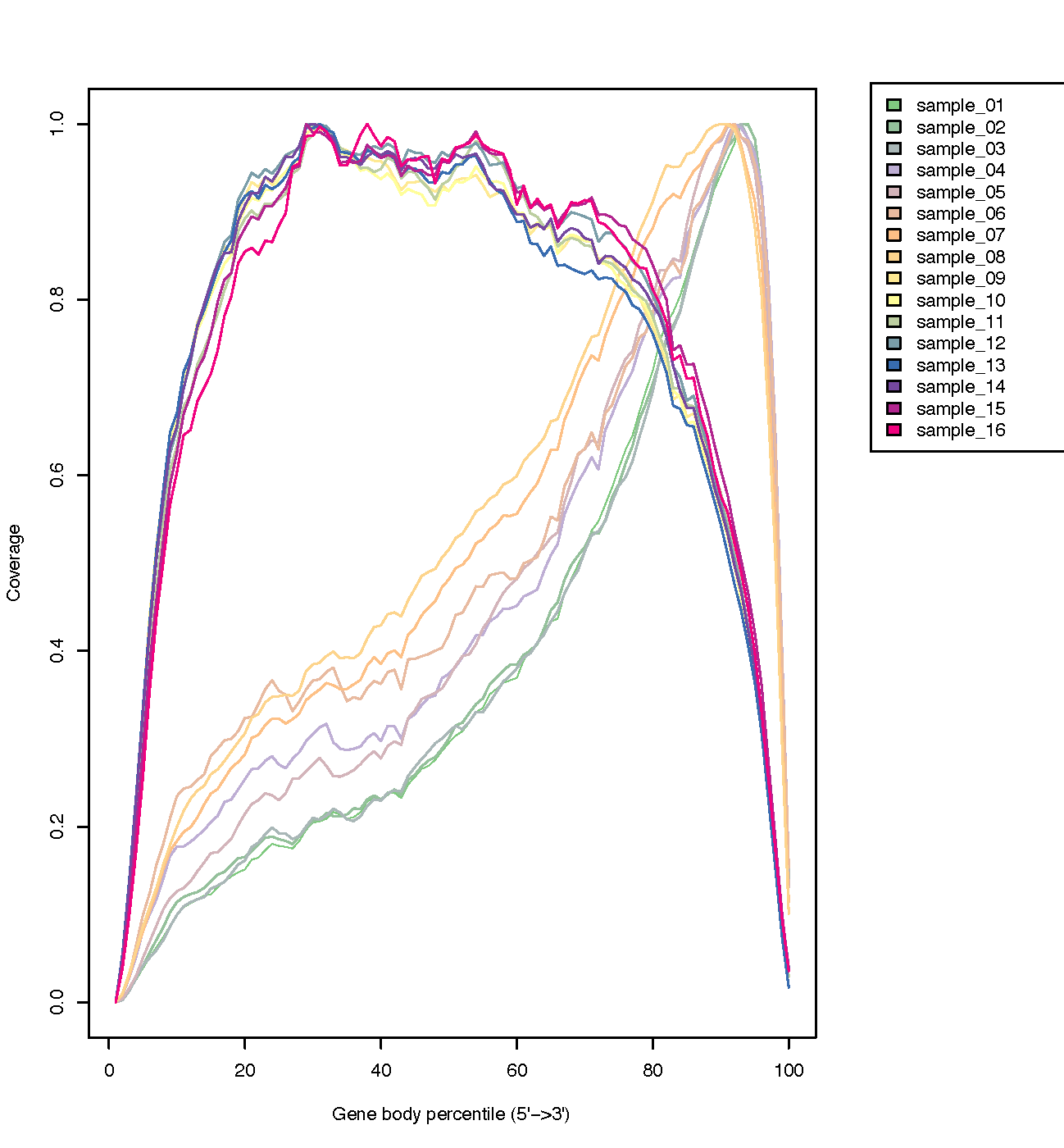
Gene Body Coverage (5’-3’)

The coverage of reads along gene bodies can be assessed to check if there is any bias in coverage. For example, a bias towards the 3’ end of genes could indicate degradation of the RNA. Alternatively, a 3’ bias could indicate that the data is from a 3’ assay (e.g. oligodT-primed, 3’RNA-seq). You can use the RSeQC Gene Body Coverage (BAM) tool to assess gene body coverage in the BAM files.

Hands-on: Check coverage of genes with Gene Body Coverage (BAM)

1. Run Gene Body Coverage (BAM) with the following parameters modified:
   • “Run each sample separately, or combine mutiple samples into one plot”: Run each sample separately.
     • “Input .bam file”: Collection of files:aligned reads (BAM) (output of HISAT2).
   • “Reference gene model”: downloaded bed file.
2. MultiQC with the following parameters:
   • In “1: Results”:
     • “Which tool was used generate logs?”: RSeQC.
       • “Type of RSeQC output?”: gene_body_coverage.
         • “RSeQC gene_body_coverage output”: Gene Body Coverage (BAM) (text) (output of Gene Body Coverage).
       • Use only flat plots: Yes.
3. Inspect the Webpage output from MultiQC.

The plot below from the RSeQC website shows what samples with 3’biased coverage would look like. Compare this with the plot you got for our dataset, which is a good demonstration of what an un-biased plot would look like.

Read Distribution Across Features (exons, introns, intergenic…)

We can also check the distribution of reads across known gene features, such as exons (CDS, 5’UTR, 3’UTR), introns and intergenic regions. In RNA-seq we expect most reads to map to exons rather than introns or intergenic regions. It is also the reads mapped to exons that will be counted so it is good to check what proportions of reads have mapped to those. High numbers of reads mapping to intergenic regions could indicate the presence of DNA contamination.

Hands-on: Check distribution of reads with Read Distribution

1. Run the Read Distribution with the following parameters:
   • “Input .bam/.sam file”: Collection of files:aligned reads (BAM) (output of HISAT2).
   • “Reference gene model”: downloaded bed file.
2. MultiQC with the following parameters:
   • In “1: Results”:
     • “Which tool was used generate logs?”: RSeQC.
       • “Type of RSeQC output?”: read_distribution.
         • “RSeQC read_distribution output”: Read Distribution output (output of Read Distribution).
     • Use only flat plots: Yes.
3. Inspect the Webpage output from MultiQC.

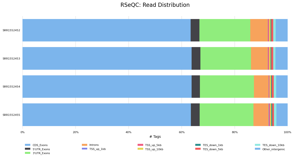
It looks good, most of the reads have mapped to exons and not many to introns or intergenic regions.

Conclusions

In this tutorial we have seen how reads (FASTQ files) can be converted into counts. We have also seen QC steps that can be performed to help assess the quality of the data in relation to its distribution on the reference genome. The next tutorial shows how to perform differential expression and QC on the counts for this dataset.

What other aspects of Quality Control could we look at for our RNAseq reads?

The reads could be checked for:

• Ribosomal contamination.
• Contamination with other species e.g. bacteria.
• GC bias of the mapped reads.
• This is single-end data but paired-end mapped reads could be checked for fragment size (distance between the read pairs). Anything else?

Key Points

• In RNA-seq, reads (FASTQs) are mapped to a reference genome with a spliced aligner (e.g HISAT2, STAR)

• The aligned reads (BAMs) can then be converted to counts

• Many QC steps can be performed to help check the quality of the data

• MultiQC can be used to create a nice summary report of QC information